
The 70% completeness of the operator count is encouraging and shows that good statistics on openings are available just by asking for the logs. Nothing special in computer facilities or staff is required: one ham can do it at home with a PC. (It does take a while though.)
Since the location of operators is not random, we cannot infer the location of the missing 30% of the operators. I'll speculate that the missing operators are more likely to be in the regions which submitted lower density of logs (the western half of the country). It's hard to imagine anyone operating in the N.E. of USA being missed in an opening like this. (This is pure speculation remember.)
The completeness QSOs, 24%, is lower. It's different (less) than the fraction of operators, since you only need to see an operator in one log to know he's in the opening, but if you don't get his log, then you miss all (but 1) of his contacts. We know that contacts occur randomly with time for 50 and 144MHz (for 220 I can't tell what's happening), so the other 76% of the contacts can assumed to be spread randomly in the temporal domain. I would expect that most of the 220MHz contacts were logged and that the missing QSO's would be more on 2m and 6m. (Again this is speculation.)
I'll assume then that the logs are a good representation of the opening. Since I don't know of any other studies like this, "good" it not precisely defined.
Caveate: the model used here has not been tested outside the data set used here. It might not be accurate. It may not even be relevant. Then on the other hand, it may be spot on - I just don't know yet.
The estimation of such numbers and the properties of the population of interest from incomplete data is a highly developed part of statistics: marketers want to sell you things you didn't know you needed, and epidemiologists find likely causes and cures for diseases. The ARRL staff assiduously tracks of the number of ARRL members, which determines whether they'll have a job next year. When it comes to tracking how much hamming is being done, the ARRL doesn't determine the number of hams who operate in its contests, whether they are getting any better at it, or if they're learning anything.
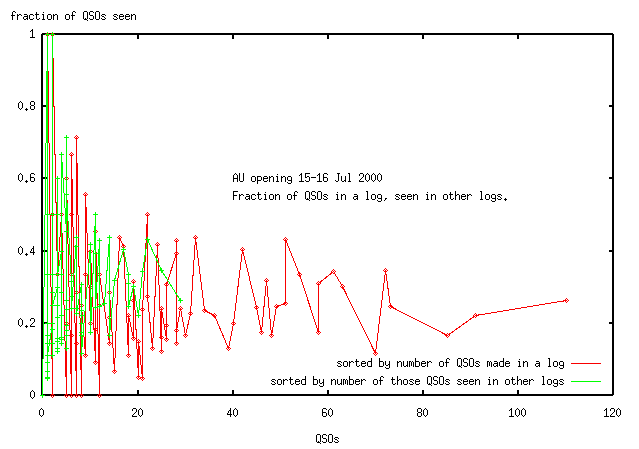
Taking the data from logs submitted with 10 or more contacts,
the reporting of QSOs is 0.24+/-0.11.
Since 2598 contacts were submitted,
then 11,000+/-5,000 QSOs were made during the opening.
Contacts with N1JEZ were not included in this calculation.
According to N1JEZ all of his contacts were Es, and none AU.
N1JEZ, operating as FP/N1JEZ from
GN16 on a DX-pedition, made 159 contacts in the time
of the AU opening, 50% more than then next highest number
of contacts in submitted logs. He would have been easily noticed in the opening.
Only 3 of N1JEZ's 159 contacts, ie 2%, were recorded in the submitted logs,
presumably because they were recognised as Es rather than AU.
It's hard to imagine that such a large number of
contacts were "missed" in the logs for other reasons,
e.g. because of a statistical aberration.
I assume operators did the same with other Es contacts.
With an average reporting of contacts=24% and a reporting
of 2% for the Es contacts of N1JEZ, then Es contacts are
(miss)reported 8% of the time.
This is an upper level since I asked for logs of the opening,
not just for the AU contacts.
Clearly working N1JEZ was a big deal for some people and they
naturally wanted to report it.
The problem then is to determine the number of hams that were were needed to produce these
extra 8,500 contacts, but who weren't seen in the logs.
There is no relation between the number
of contacts and the number of operators in an opening, that I know of.
It's quite possible from this data that the 700 people seen account for all the contacts.
The people who sent in logs made an average of 2500/111=23 QSOs.
We could make the assumption that those who didn't send
in logs make a similar or a lower number of contacts.
The remaining 600 people then would need to account for the 8,500 extra contacts,
an average of 14 contacts each, a number which is compatible with not needing any more hams.
The lower bound for the number of extra hams then is 0.
This calculation gives no information on the upper bound of number of operators.
For the AU opening,
you ask volunteers to report who they see (contact)
by inspecting their logs for contacts.
You then plot the frequency distribution of the number of times
each of operators were detected.
In the experiment here,
the volunteers (i.e.the people who sent in their logs)
took 2598 samples of the opening.
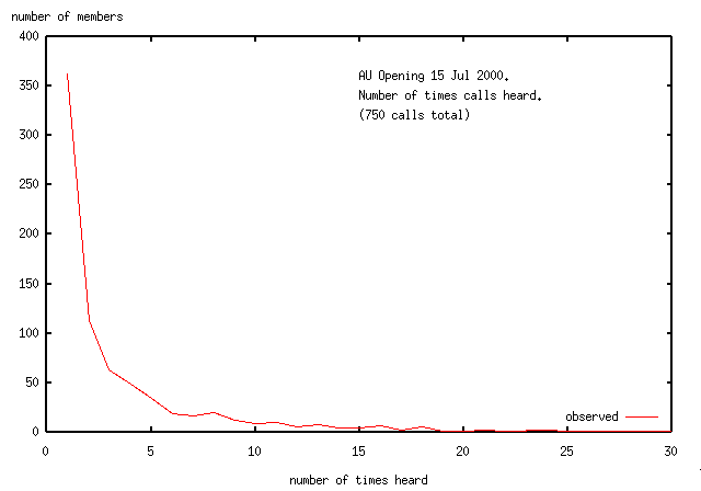
The following shows the frequency distribution for contacts in the opening
i.e. the number of operators (y) who were contacted (x) times.
For instance 362 hams (about half of the calls worked) were seen/contacted once,
while 34 of the participants were contacted 5 times.
To analyse this data, I needed a model of how hams make contacts.
To have somewhere to start, I made some assumptions about the data:
As Rodney Dangerfield would say
"how untrue are they?"
It is reasonable to assume that a large enough number of different processes,
when added together, will have the same statistics as a random process.
It is conceivable then that a large enough number of observers,
spread over a respresentatively large area,
will see the whole opening as a set of random contacts.
In this case the assumptions made above
would be sufficiently true to determine the number of people missing from the logs.
(This assumption fails as we see below.)
If contacts are made randomly and there were 2500 hams operating during the opening
and we took 2500 samples (i.e. recorded 2500 contacts),
then most of the time we would be observing different operators.
The distribution then would show many operators observed
only once and a few would be observed several times.
Some would not be seen at all.
If instead there were only 500 operators and recorded 2500 contacts,
then we expect that an operator would be oberserved
an average of 5 times, i.e. there would be a peak
at x=5 and few operators would be seen 1 time or 10 times.
Let's test these assumptions.
This first attempt at a model (which fails), has CQs going out (the identity of the
calling ham is not recorded) and a ham is selected at random to answer the call.
All participants have an equal chance of making a contact.
We saw 700 or so unique calls in the sampling (200 or so of which may
be bogus), so we know that the population of operators in the opening was at least 500.
The simulation was run for the number of operators in the range 100-3000.
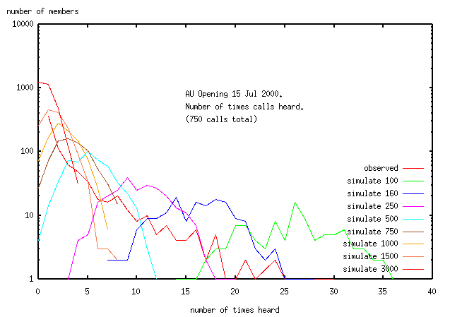
Here is the simulated and observed frequency distribution
plotted on a log-linear graph,
for an opening in which 2577 contacts were made.
(The name of the distribution used in this simulation is "Poisson").
It is clear that the Poisson distribution
does not fit the observed frequency distribution for any
(reasonable or unreasonable) hypothetical population size.
The line for the observed data is a (jagged) straight line,
while the simulated data are (jagged) bell shaped curves.
Compared to model, some of the population is making more
contacts than expected (the tail on the right of the graph).
The strategy for this is well known:
get a stable, well paid job so you can get a good location,
and don't have to move every 2-5yrs,
put up towers and spend all your time and money building gear
and improving your operating skills.
Some of the population are making less contacts than expected.
A subset (upto 200 people) has found a way of only being
seen once in the opening (the tail on the left hand side of the graph).
The strategy to acheive this isn't obvious.
There could be 200 people making only one contact because they
are waiting for an operator to appear from a rare grid
(unlikely - there aren't operators in 200 rare grids).
Another explanation is that these 200 people aren't real -
they're bogus (miscopied) call signs (i.e. almost half of the
calls heard or 10% of the contacts are with invalid calls).
Yet another explanation is that AU is just beyond the reach of most
operators and many are doing well to get one contact and they
take all night to get that one.
For myself, the first time I operated in the EME contest I
only got 1 contact on 2m (needing both weekends for that)
and the next year only got 1 contact on 432 (this taking all of the first weekend).
Possibly there is a very large resevoir of people just on the edge
of being able to work AU and who only appear in a big opening like this.
This possibility is explored further below.
Hams then are not making contacts randomly.
The frequency data ranges over 2.5 orders of magnitude in (y)
and drops off faster than exponential,
not resembling a Poisson distribution at all.
We need a new (non-random contact) model for the opening,
in which case we need a better understanding of the way hams operate.
Surprisingly such perfect data is available:
the subset of contacts made between the hams who turned in logs.
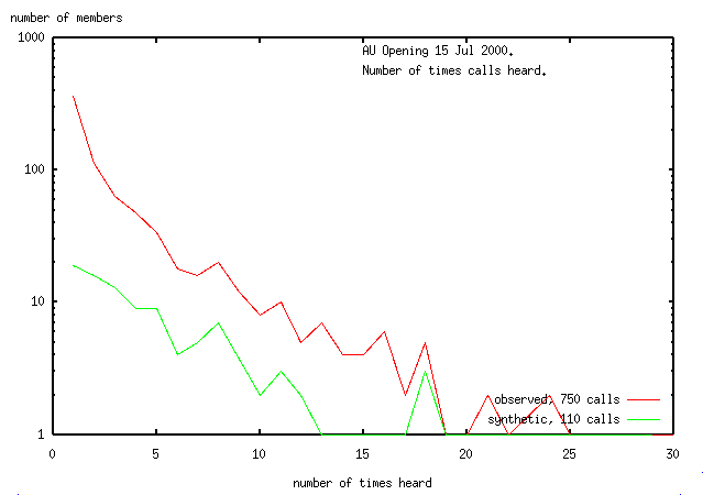
Their synthetic mini-opening consists of 626 contacts, and 111 operators.
I assume that the contacts they made with operators in the greater contest did not
interfere with their contacts in the mini-opening.
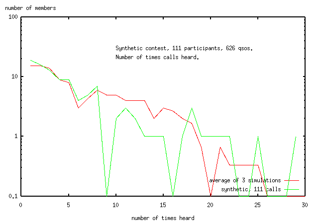
Here's the frequency distibution for the synthetic data
(Because of the log plot, data <1 is truncated to 1).
The data from the whole submitted log is included for reference.
The line for the synthetic data has no upturn for
the singletons (operators seen only once), supporting the evidence from
analysing the gridlocators
that about 200 of the singletons observed in the opening are bogus.
For analysis of the logs, the number of operators seen was changed to the
value determined above (571).
The contacts cuurently assigned to the 177 bogus
calls should be should be reassigned to other bins,
but there is no information on how to do this - the contacts were just discarded as invalid.
Both lines are emperically fitted by the equation
number of members = k*e^(-0.2*times heard)
In the (failed) poisson fit to the 2598 QSOs (above),
operators are selected randomly to make a contact.
(In fact they are randomly offered the opportunity to make a
contact and all take it i.e. with the same probability = 1).
The new model allows each operator to have different probabilities of making a contact.
The operators in the synthetic mini-contest were initially simulated by dividing the population of
operators into 10 equal sized groups,
and the members of each group were assigned a probability of making
a contact when the opportunity was offered.
This probability includes a whole range of factors,
e.g. another operator jumping in front of you, the other guy
can't copy your signal, you are listening on the wrong frequency,
you are behind a range of hills..., none of which can be separately
modelled here.
Running the simulation consisted of picking a population
size (number of contestants),
and setting probabilities for each of the 10 groups.
Then an anonymous entity starts calling CQ to all in the contest
(the identity and location of the calling operator is not
of interest for this simulation and is not recorded).
An operator is selected randomly to intercept the CQ
(here called a contact opportunity),
the probability assigned to that operator for making the contact
is looked up and the result (QSO made or missed) is recorded.
The simulation continues, offering contact opportunities
to randomly selected operators till 626 contacts (the whole
synthetic contest) are recorded.
The calculated contact frequency distribution
and number of operators seen is compared to the observed observed data.
(Alternatively the simulation could have proceded till
111 operators were seen and the number of contacts made
could have been compared to 626).
The assigned probabilities are in fact relative rather than absolute.
The best operators is assigned a probability of 1.0
and the others lower probabilities.
If the probabilities of each group had been reduced by the same
factor (eg by 2) then the simulation would produce the same
contact frequency distribution and number of contestants seen,
but more contact opportunities would have been needed
to get the same number of contacts (i.e. more contacts
would be missed).
Thus the simulation has 11 variables, 1 for population and
10 for probabilities. One might think (as I first did) that you
could fit anything with 11 variables and that the values
of each variable would not be independant (ie you could fit
any population size you liked by changing the probabilities).
As it turns out not all probability distributions are
independant -
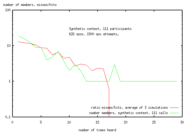
The next figure shows the number of contacts that were missed to make one contact.
About 1550 QSO opportunities were required to make the 626 contacts,
ie the average ham who sent in a log requires 3 times as many opportunities
as the best hams to make a contact.
The worst off hams only get 1 contact out of 15.
(Not all of this is neccessarily due to skill.
The average ham probably has a worse location than
the ham who makes all his QSOs, and the hams in western USA
are all in worse locations VHF-wise than those in NE USA.)
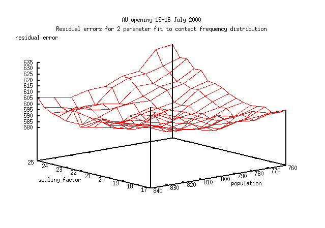
Some improvements were made to the model.
probability(member_number) = e^-sqrt(scaling_factor*member_number/total_popln)
This empirical equation was incorporated into the model giving a 2-parameter
(population, scaling_factor) fit, rather than 11 parameters.
As before, each time the simulation was run, a member of the population was chosen randomly.
Let's say member 525 (of a total population of 571 hams) was picked.
The probability for ham 525 of completing the contact would be calculated
p(525)=e^-sqrt(scaling_factor*525/571)
Then a random number generator would determine if ham 525 made or missed the contact.
The result would be recorded. The process is then repeated.
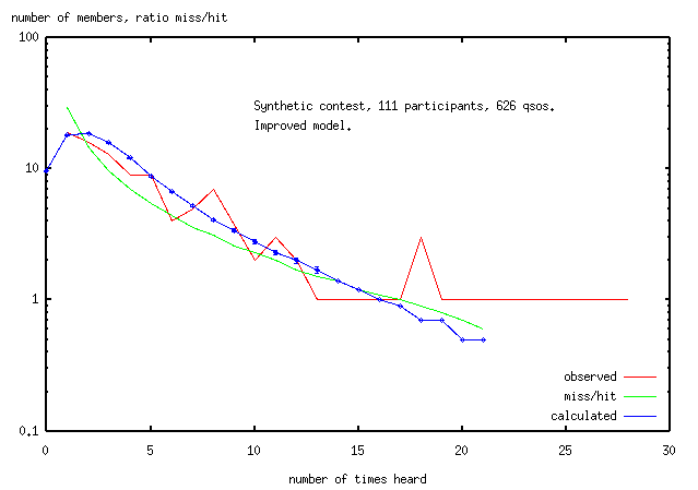
In the synthetic (perfect) contest, the number of people
who were contacted 0 times is 0 ie freqdist(0)=0.
The simulation calculates the number of unobserved people, freqdist(0)=11.
There is no reasonable fit to the synthetic dataset for which freqdist(0)=0.
For the data to have the maximum value at freqdist(1) and freqdist(0)=0
then many high order terms (which we don't have) would be needed.
Either the model is wrong or there is something strange about the synthetic dataset.
The synthetic dataset was produced by truncating a real data set and not from a
real perfect contest in which all logs were submitted
(including by those who didn't make any contacts, but who wanted to).
Possibly some unobserved people should have been carried over into the synthetic contest.
Even knowing that a discrepancy exists between the data and the model,
it is not obvious whether or not the synthetic data is valid.
The real data does expect a finite value for freqdist(0) which is provided by the model.
This statistical issue requires someone who knows more about statistics than I do.
For the moment I will assume that the perfect data set has some abberation arising from
the truncation used to produce it.
I also assume that the calculated freqdist(0) to fit the observed data
is the number of unobserved people in the contest.
(One problem is that freqdist(0) comes from extrapolation of a poorly tested model.
That I'm prepared to do this should convince
even the least sceptical of you that I'm up to no good here.)
The observed data (integers)
is quite noisy compared to the average of 512 simulated
contests (which are floating point)
and most of the data is outside the calculated errror bars (later found to be a mistake in
my program, which was corrected for the real data of 2598 QSOs in the next section).
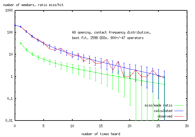
The calculated ratio of misses to hits for the operators getting the
least number of contacts is about 30:1.
Monte Carlo simulation of the errors in the number of operators gave:
number of operators=121+/-1 (for number of Monte Carol runs=6).
The real data is assumed to be valid for people who were worked 2 or more times.
The first problem is to determine the real number of people who were only worked once.
The logs give 361 for this, but many of these operators are bogus.
There are 2 (relatively independant) estimates for this number.
With this information the model can be fitted to the real data.
There are still some practical problems with fitting the model to the observed data
Such convergence problems can sometimes be fixed by reparameterising the problem.
This approach will not give better fits or result in different estimates of
the original parameters, but will allow faster convergence.
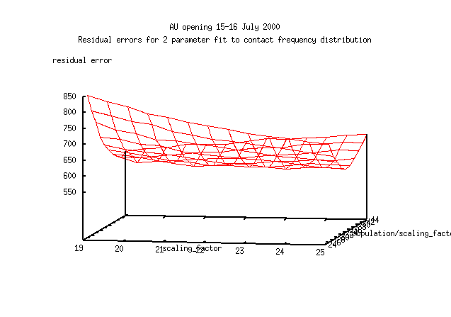
Here's my first attempt at reparameterising the
estimating funtion (parameters: scaling_factor, population/scaling_factor).
The viewing angle shows a valley with nearly constant depth for large
changes in scaling_factor and a slope comparable to the noise in the
calculation. This is no better a parameterisation than is the previous one.
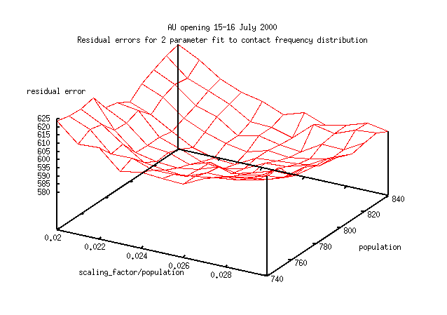
The valley is now nearly parallel to one of the axes, meaning that the
two parameters are no longer strongly correlated.
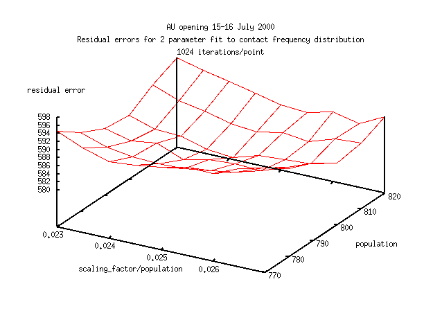
Here's the next attempt (which works). The new parameters are (population,
scaling_factor/population). For the same percentage change in parameter,
the slope is large compared to the noise, and the estimates of the parameters
are not correlated.
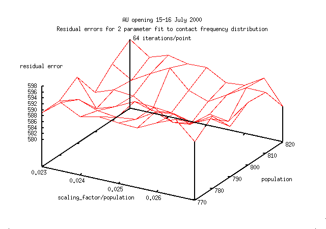
The next problem is to determine how many iterations are needed to reduce the
roughness of the error surface so that you can reach the best fit point well
within the radius of the expected standard deviation of the parameters.
The problem with this is that you won't know the variance of the parameters
till after you've done the fit.
However the
estimates of freqdist(1) shows a range of 20, so a standard deviation
of 5 is a reasonable first guess.
Hopefully you will be able to calculate the fit to this degree of
resolution in a convenient time.
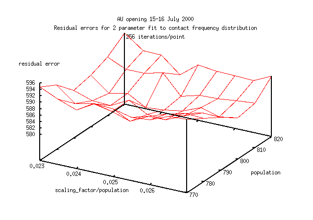
Here are 3 error surfaces calculated with 64,256 and 1024 iterations for each
point on the surface (1024 iterations or 1 point on this figure,
takes about 30mins on a 300MHz 32bit machine).
The images are a smaller part of parameter space than shown immediately above.
Notice how the error surface becomes smoother with a larger number
of iterations.
A good estimate (standard deviation of population = 5)
of the point of best fit isn't clear with until you reach 1024 iterations.
Here's the best fit (scaling_factor/population,population)=(0.025,800),
from 1024 iterations. The error in the number of operators was determined
by Monte Carlo simulation (below) and is included here for convenience.
The miss/hit ratio is offset by 0.05 on the x-axis for clarity.
The program which does the fitting is
available with the whole download or is available here,
simulate_4.pl.gz.
Brief reminders of the program's usage are in perldoc format.
The main information on its use are in this section.
The operators showed a 30:1 range in ability to make contacts.
Although in the model it is not obvious where this number comes
from, intuitively it comes about because all operators (on average)
are offered the same number of contacts. The best setup operators
make all of the contacts offered to them (by definition),
which in the data is 30 contacts (as seen in other logs).
Thus the worst setup operators we see (who
get 1 contact) will miss 29 contacts.
Why does this model fit, when we've assumed that hams make contacts randomly
with each other, when we know that
they don't.
It's because in this model, the chances of an operator having a 2nd contact with
one of 800 other operators when only 2598 contacts are made, is quite small.
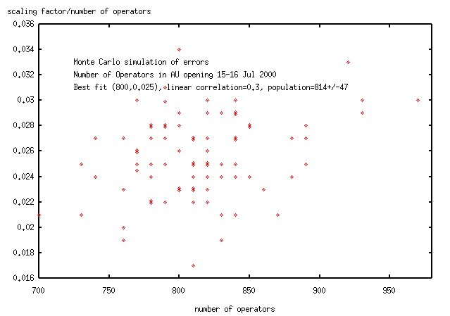
Here's the Monte Carlo simulation of errors (this took a month on a 300MHz computer).
The linear correlation co-efficient of 0.3 means that 0.3^2=10% of the variation
in one parameter is due to variation in the other parameter. I'm going to take this
to indicate that the parameters (population, scaling_factor/population) are uncorrelated.
The
equation
which produces the expected contact frequency distribution is not linear
with respect to population size.
We would not expect the distribution of estimates of population size to be normal.
If the distribution of the estimates of population is assumed to be normal,
then (mean,s.d)=814+/-47 (the best fit is at population=800).
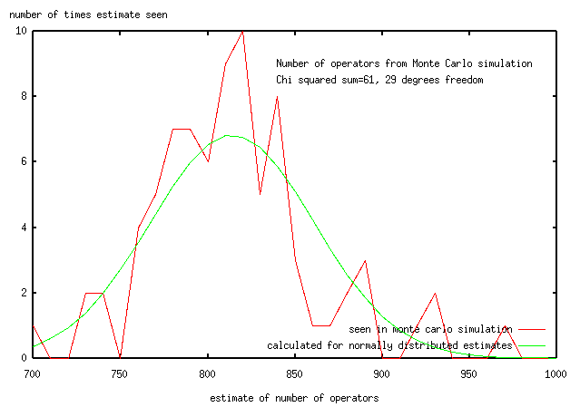
Here's the distribution of population estimates,
along with a normal distribution with (mean, s.d)=814+/-47 which has the same area.
The Chi squared sum is 61,
indicating that the distribution of estimates is not normal at a 1% level
(i.e., there is less than a 1% chance that a normal distribution
of errors would produce the red curve).
The normality or otherwise of this distribution isn't of concern here.
If it's normal, I can give a standard deviation for the best fit.
Since it's not, I can just give estimates for the +/-34% level.
In the whole opening, the 11,000 contacts were made by these 800 operators in about 4hrs,
an average of 14 contacts each.
(C) Joseph Mack 2000-2002, Joe NA3T, jmack (at) wm7d (dot) net, http://www.wm7d.net/azproj.shtml
Previous
Next
Table of Contents
Number of Operators
Sampling is a method for determining properties of a large
population. You can determine the number of bats in your
neighborhood or number of birds migrating each year along the
(US) eastern fly-way by sending off an enthusiastic bunch of volunteers to
capture, tag and release a large enough number of the chosen animal.
When you've finished, you count the number of different individuals seen
and plot the frequency distribution (number of times individuals were captured n times).
So if 50 particular individuals were each seen(captured) 10 times and a different group
of 100 individuals were each seen 5 times, then freqdist(10)=50 and freqdist(5)=100.
Using a model for the sampling (in this case, individuals are captured randomly)
you can determine the number of birds migrating on the US eastern fly-way.
Obviously neither of these assumptions are true.
Here are the problems:
Analysis of a Perfect Data Set for a Ham Contest
There are no models (that I know of) for the number of QSOs as
a function of number of hams and time in a ham contest.
If I were to propose such a model, I would need a set
(or many sets) of good/perfect data to test it.
The data would come, of course, from contests where all
participants turn in logs, all QSOs are recorded and all
submitted gridlocators and callsigns are correct.
As I realised later (see below),
the people who tried to make contacts, but didn't succeed,
would also have to turn in logs.
Large misfits are obvious by inspection.
Here's the simulation for 111 operators, 626 contacts
(Note:Some of the data and calculated points have value zero.
These are truncated to value 0.1 by the log plot.
This truncation makes visual checking of the fit a little confusing.
The worst discrepancy is at "number of members"=13, where data=1, fit=3.)
Here's the fit to the synthetic dataset using the improved variable probability model.
(This number is <1.0).
Analysis of a Real Data for the 15-16Jul2000 AU opening
With a model that shows promise for fitting the AU opening, the next stage is
to analyse the real data.
Only the first estimate is independant of the probabilistic model
and was used as the value for freqdist(1).
However we now have an estimate for the range of freqdist(1) - from 158-177.
Here is the error surface for the fit in its current parameterisation.
Ideally you would like the surface to be a paraboliod of revolution
so that the values of the two parameters would converge quickly.
The surface is more like a piece of paper, picked up by 2 diagonal corners.
The estimates of both parameters are correlated and the surface is rough
compared to the slope near convergence.
With a function for the calculation which is expensive to calculate, it will
be difficult to fit this data
(I spent about 2 weeks using this parameterisation,
before realising that I was getting nowhere).
Conclusion